

An End-to-End Comprehensive Summary of Machine Learning
A cheat sheet for machine learning concepts and practical implementation tips
Introduction
If you are new to the machine learning world and want to get your feet wet super-fast in all the concepts of machine learning without getting overwhelmed by the mathematical intricacies involved in the background, then read this.
This article contains key concepts of machine learning put together based on the knowledge I acquired from multiple sources especially from Prof Andrew Ng’s Machine Learning online course and in-class lectures with links for further reading for those interested.
I hope this can serve as a go-to spot for new-machine learning enthusiasts and also those who want to refresh their minds on what is machine learning with some critical implementation tips.
Please bear with me this post is a little lengthy but it’s understandable and worth your time as it touches almost every major concept in machine learning.
The article is sectioned into days just for those who might love to take things slow. You can read a day’s highlight then try researching further and implementing a project based on the concepts. This gives it structure.
So without wasting much of your time, let’s get to it.
DAY ONE HIGHLIGHTS

image from Coursera
Introduction.
Machine Learning is a branch of artificial intelligence that provides computer systems the ability to automatically learn and improve from experience without being explicitly programmed.
It is broadly divided into 2 main categories: Supervised and Unsupervised. Also, we got Anomaly Detection Problems that incorporate supervised and unsupervised techniques.
Supervised Learning.
In supervised learning, a learning algorithm(model) is trained with labeled data. The machine learning algorithm (model) learns from this labeled data through an iterative process which then enables it to perform predictions on new unseen data.
Supervised learning is further divided into Regression and Classification Problems.
Linear Regression Analysis.
In a regression problem, the output variable to be predicted by the model is a numeric value. For example, predicting the price of housing in New York City or maybe predicting the amount of energy consumed by a certain state.
The objective of Linear Regression.
In linear regression, the objective is pretty straight forward.
Given a labeled training set of m-training examples the objective is tofind model parameters that minimize the cost function. This will be made perfectly clear shortly.
Regression can be univariate or multivariate.
Univariate Linear Regression.
Univariate simply means a single variable (feature). A regression problem where the input examples, X(i) used for training a linear regression model is a single value or 1-Dimensional vector is a Univariate linear regression problem.
Here is an example of a labeled training dataset with a single variable(age) and corresponding output(weight). Given only the age of an individual, the model aims at predicting the weight of the individual.
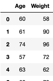
image univariate dataset
Technically, the figure below summarizes a linear regression model. In this case, it is a univariate model as the X is a value and not a vector.
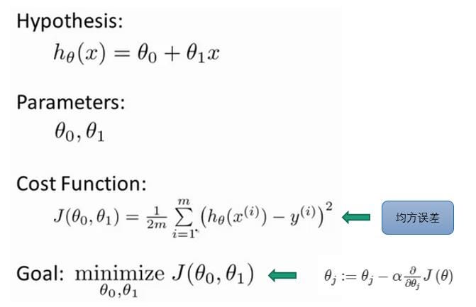
source: ProgrammerSought
The question that arises is,
How can we find the values of model parameters(thetas) that generate the minimum value of the cost function?
Luckily Gradient descent comes in to save us the headache.
Gradient Descent
Gradient Descent is a general algorithm that is used to minimize different types of functions. In linear regression, we use a gradient descent algorithm to automatically and simultaneously update the model parameters.
It is an iterative algorithm. For each iteration, the derivative of the cost function is evaluated and the model parameters are updated. This is done until hopeful convergence of the cost function is reached i.e the global optima is found.
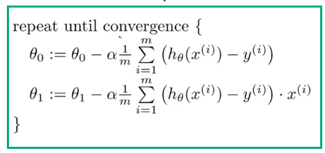
Gradient Descent Algorithm
Two fundamental things that make up the gradient descent algorithm is the learning rate and** partial derivatives of the cost function.**
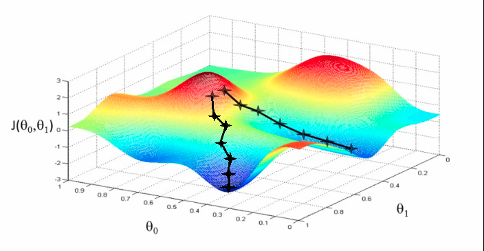
Illustration of Gradient Descent: Source: Coursera
The learning rate(alpha) also determines how much of a step size we take when updating model parameters. The partial derivative term indicated by the summation term above gives the direction of the steepest slope.
SideNote: Remember that, the derivative of a function at a particular point is the slope of the line tangent to the function that passes through that point.
Key Note for Gradient Descent
If alpha hyperparameter is too small, gradient descent becomes too slow, as it takes a lot of time to converge to a local minimum. This is because the updated theta-parameters are increased by tiny baby steps down the hill.
If the alpha is too large, we might overshoot and even diverge. That is we might jump over the minimum value and never converge.
This gradient descent algorithm explained here is also known as **Batch gradient descent, **as the algorithm uses all the training samples in each update iteration process of the model parameters.
Here are links to some articles including mine to broaden your understanding of the basic concepts
Linear regression detailed view article on medium by Saishruthi
DAY 1 DONE!!
** DAY TWO HIGHLIGHTS **
Linear Regression with Multiple Features
When we have more than a single feature in our training data for each training example to use for prediction, each of the training examples now becomes a vector instead of a single value. To be specific, in such cases, each training example becomes an n-dimensional feature vector where n = number of features in the training set.
This is known as multivariate Linear Regression. Multivariate simply means multiple variables or features. An example dataset is shown below where the number of features, n, for each training example is four(4) and the labeled output is the salary increase.
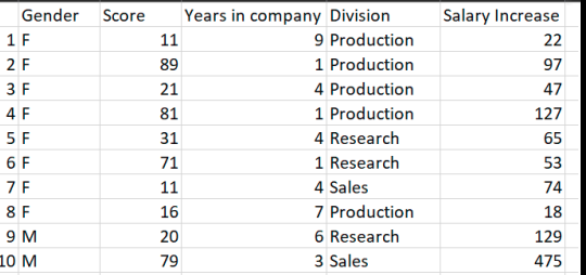
Image of training dataset with multiple features
The hypothesis for the multivariate linear regression is an extension of the univariate linear regression shown below where n = number of features.
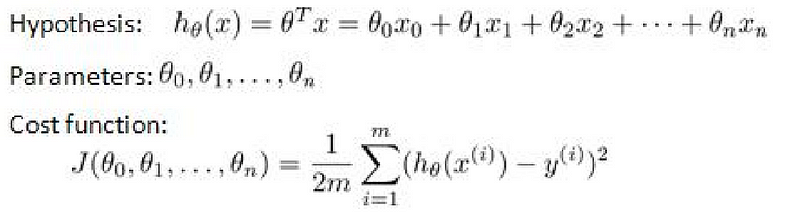
Multivariate linear regression hypothesis and cost function
What this means is that a unit change in feature i, corresponds to a change, bi in the hypothesis. E.g price of houses.
In Gradient Descent for Multivariate Linear Regression, the cost function J, simply changes by the number of model parameters(theta), as seen in the figure above.
In regression, we often add a regularization term to the cost function which helps us avoid overfitting our model as seen below. More on this can be found on additional links I will share at the end.
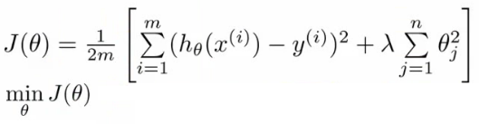
Cost function with regularization term.
Feature Scaling
It is one of the 2 common techniques that aims at adjusting the ranges of all features to be the same or close to each other.
Feature scaling helps the gradient descent algorithm to converge much more faster and with fewer iterations and also correctly. If the range of values is too small, scale up and scale down otherwise.
Mean Normalization
It is another technique mostly used for feature scaling.
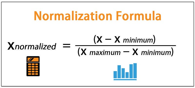
Image by wallstreetmojo.com
Determining when Gradient Converges.
Plotting the cost function, J(theta) against the number of iterations performed by the gradient descent algorithm is a good practical way to determine if gradient descent has converged.
A small value of learning rate results in a very slow convergence i.e it takes so much time to reach the global optimum of the cost function.
On the other hand, if the learning rate is too large, the cost function may not decrease on every iteration and can even diverge
Normal equation Technique
It is a technique used to solve for the values of the model parameters which minimizes the cost function analytically. It doesn’t perform an iterative process like gradient descent and we do not choose any learning rate.
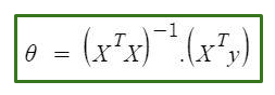
normal equation formula
For a very large number of features i.e n = 10000+ the normal equation becomes computationally expensive as we need to compute matrix inverse which is quite an expensive process for large matrices. In this case gradient descent is the best choice.
Key Note
If the X.TX — matrix of the normal equation is non-invertible i.e it is singular or degenerate, then this implies 2 main things
- Redundant Features — Linearly dependent Features\
- Too many features
Here is a good article on feature scaling.
DAY 2 DONE!!
** DAY THREE HIGHLIGHTS **
Classification

In classification, the objective is to identify which category an object (input) belongs to. For example, we can be interested in determining if an image contains a dog or cat, color red or black, email spam, or genuine, a patient has HIV or Not.
A very common model used to solve classification problems in machine learning is Logistic Regression.
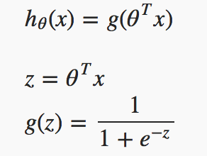
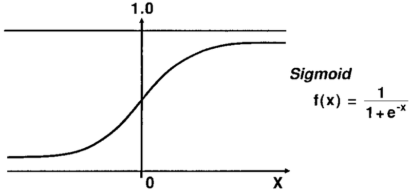
Logistic Regression
It is a classification algorithm that is based on the sigmoid or logistic function whose values are squashed between 0 and 1.
Source: Researchgate.net
h(x) = g(z) as seen in the image above is the hypothesis function or sigmoid function used to compute output values or probabilities within the range 0 and 1.
The way our logistic function behaves is that, when its input, z, is greater than or equal to zero, its output g(z), is greater than or equal to 0.5:
Binary Classification
In binary classification, the output is either 0 or 1, so it is necessary for the hypothesis to also be within the range 0 and 1 contrast to the case of linear regression. That is why we use the logistic or sigmoid function for the hypothesis.
It is often interpreted as a probability.
For example, let’s say the output value of the hypothesis, h(x) for the case of a ham or spam email classification problem is h(x) = 0.7, where 0 represents ham email and 1 represents spam. This simply means that there is a probability of 0.7 that the email is spam.
Decision Boundaries
It is a boundary that separates the dataset into its various classes. In a binary classification problem, the decision boundary is the line that separates the positive examples from the negative examples in our dataset.
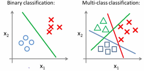
image from medium
Non-linear decision boundaries can also be used in classification tasks to obtain better models.
Cost Function For Logistic regression
The cost function for Logistic regression is different from what we have seen in linear regression. This is because if we use the cost function of linear regression in evaluating the logistic regression model, it will result in a wavy and irregular form with many local optima i.e it is not a convex function.
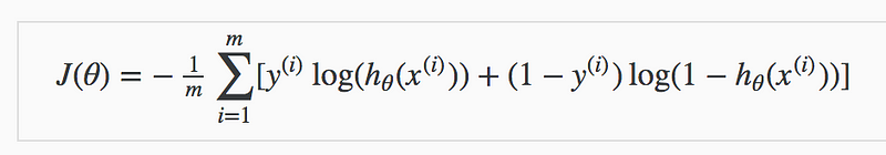
The cost function for logistic regression
Multiclass Classification
We use the one-vs-all(or one-vs-rest) classification technique whereby we train n-binary logistic classifiers for the n different classes in the dataset.
This is achieved by setting the class labels of a single class to positive and then the labels of the other training examples belonging to the rest of the classes to negative during training. This is done in turn until we have train n-binary classifiers for the n-classes in our dataset.
During prediction, the input is run across all n-classifiers. The input belongs to the class whose model outputs the highest probability.
Solving the Problem of Overfitting.
Underfitting also called high-bias occurs when we have very minimum data for training.
Overfitting, also known as high-variance often occurs when we have too many features in our dataset.
There are two main options to address the issue of overfitting:
- Reduce the number of features:
We can reduce the number of features in 2 ways
- By manually selecting which features to keep.\
- By using a model selection algorithm.
Regularization works well when we have a lot of slightly useful features.
** DAY 4 HIGHLIGHTS **
Neural Network and Representation.
Neural networks were developed as simulating neurons or networks of neurons in the brain. The image below shows the fundamental structure of an artificial neural network.
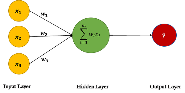
image of a single artificial neuron
Each circle is called a node. The yellow nodes are known as the input nodes(features). The green node is called the hidden node and finally the output node in red. These hidden nodes(units) are commonly referred to as activation units as the functions which they compute are called activations functions. The most common activation functions are sigmoid and Relu(Rectified Linear Unit)
By stacking these nodes in a structured manner we can create very powerful models that are capable of performing complex tasks with high accuracy. The image below shows a three(3) layer neural network(input layer is not counted).
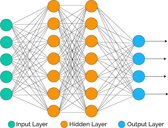
Image of 2 layers neural network from Towards Data Science
Applications of Neural Networks
Neural networks are versatile and therefore can be used for many different applications. They are used for binary classification as well as multiclass classification tasks. Neural networks are also used to solve regression problems.
Here are some practical use cases: Character recognition, Image compression, prediction problems such as stock market prices, signature recognition, and a lot more.
Links for more information on neural networks is included at the end of day 5. Keep going.
DAY 4 DONE!!
** DAY 5 HIGHLIGHTS **
Neural Networks: Learning
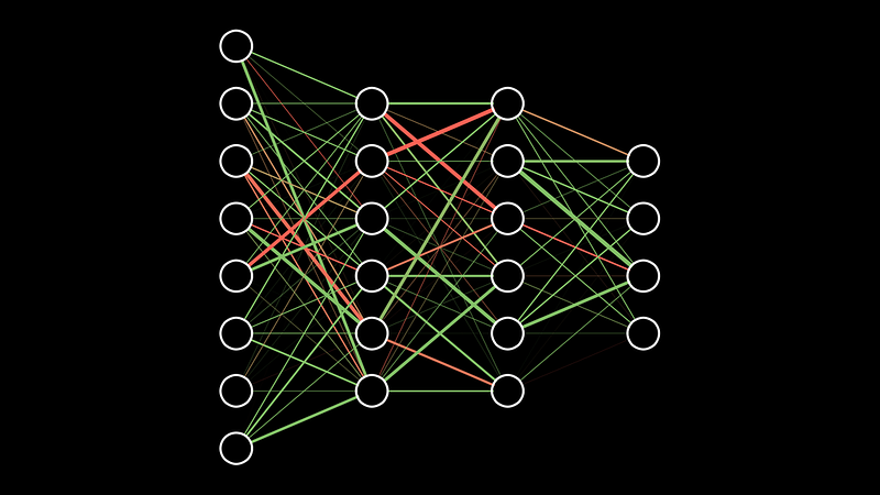
Image from 3blueOneBrown youtube
A Neural Network is one of the most powerful supervised learning algorithms. In machine learning problems, It is often good practice to train neural network classifiers when a linear classifier doesn’t work.
Training a Neural Network
Training a neural network is an iterative and computationally expensive process which involves finding the best model parameters — weights and biases that minimizes the error.
The driving mechanism behind finding the best model parameters is based on an algorithm known as Backpropagation.
SideNote: Neural networks are actually very complex and very mathematical, so I won’t dive deep into that here.
Back Propagation algorithm.
Backpropagation is the algorithm that is used to find the optimal model parameters i.e weights and biases of a neural network based on the training data in an iterative manner.
It does this by computing the partial derivatives of the cost function, J with respect to the weight and bias values.
Backpropagation together with the cost function is used by the gradient descent algorithm to evaluate the optimum model parameters. This is the training phase of a neural network and it results in optimal model parameters.
Gradient Checking is a method that is used to verify if the implementation of backpropagation is working properly.
Bias Vs Variance
In training a neural network, we need to first decide on the network architecture. The network architecture is simply, the connectivity pattern between neurons, i.e the choice of the number of hidden layers to use.
Note that the number of input units to a neural network is equal to the dimension of the features of training examples. If you are dealing with a classification problem, the number of output units is determined by the number of classes.
It is also great practice to use the same number of units in every hidden layer in your neural network. The greater the hidden units the better performance of the model but increase in computational complexity,
Steps to Training a Neural Network
1. Randomly initialize the weights
2. Implement forward propagation to obtain the output value for each training example.
3. Compute the cost function
4. Implement backpropagation to compute partial derivatives
5. Use gradient checking to confirm that your backpropagation works. Then disable gradient checking.
6. Use gradient descent or any built-in optimization function to minimize the cost function by iteratively updating the weights and biases.
Note: When implementing neural networks we do not initialize the model parameters with zeros, as the model does not learn any interesting features after training. This is called the symmetric weight problem. Random initialization of the model parameters is performed to avoid this drawback. This is called symmetry breaking.
For more Information on Neural Networks, here are some important links.
- Tony Yiu’s article gives an intuitive explanation of the process behind neural networks (see here).
- If you want to take it a step further and understand the math behind neural networks, check out this free online book here.
- If you’re a visual/audio learner, 3Blue1Brown has an amazing series on neural networks and deep learning on YouTube here.
DAY 5 DONE!!
** DAY 6 HIGHLIGHTS **
Debugging a Learning algorithm
If your trained machine learning model is performing poorly on test data, here are some general steps you can try to improve the performance of the model.
- Get more training examples\
- Try smaller sets of Features\
- Try getting more additional features\
- Try polynomial Features\
- Decrease or Increase the lambda of the regularized term
Evaluating a Hypothesis
Traditionally, to evaluate how well a model is performing, we split the data into training and test split. We then train the model using the training split to obtain the optimized model parameters(thetas).
Using the trained model parameters, we evaluate the test set error using only the test split examples. This gives us an idea of the performance of your model on unseen data. This technique is often applied to regression problems
Misclassification error is another metric that is often used to evaluate how well a hypothesis is performing for the case of classification.
Generally, it is good practice to split data into train, cross-validation, and test set. This helps to provide an unbiased evaluation of a model fit on the training dataset while tuning model hyperparameters.
Model parameters are computed with the training set, then the cross-validation set is used to evaluate the model performance i.e if model might be underfitting or overfitting or not. Hyperparameter tuning or other changes can then be made and the model re-trained and tested using the validation set.
Rule of thump.
Choose a model with the least cross-validation error, then using the test set, compute the test error(J_test) to choose the model with the least test error.
Bias Vs Variance
If your trained model performance is quite low, it could be as a result of either high bias(underfitting) or high variance(Overfitting).
To identify which of these your model is suffering from, check the error on both train and cross-validation set.
If train error and validation error are both high, it implies the model is underfitting(high-bias). If training error is low while validation error is** high,** it means the model is overfitting(high variance).
Learning Curves
Use Learning curves to diagnose if your learning algorithm is suffering from a bias or variance problem,
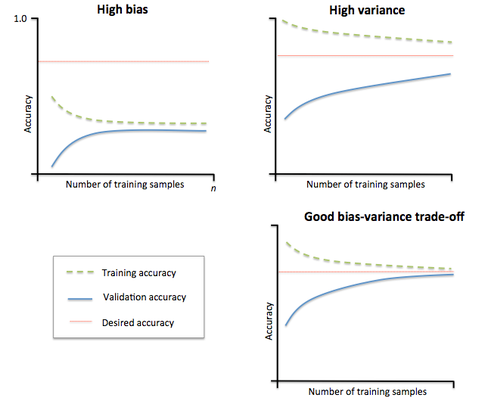
Image if high bias(low variance), high variance(low bias) and Good bias-variance tradeoff
If your algorithm is suffering from high bias, increasing the training examples doesn’t help reduce the training and cross-validation error value.
Conversely, if your learning algorithm is suffering from high variance, getting more training examples can likely help improve its performance as, cross-validation cost error will keep decreasing with more training examples.
Final Decision Process for Machine Learning Model
Our decision process can be broken down as follows:
1. Getting more training examples: Fixes high variance
2. Trying smaller sets of features: Fixes high variance
3. Adding features: Fixes high bias
4. Adding polynomial features: Fixes high bias
5. Decreasing λ(regularization hyperparameter): Fixes high bias
6. Increasing λ: Fixes high variance.
Evaluation Metric For Classification Models.
Precision and recall are good evaluation metrics for classification models as it can help pinpoint the effect of skewed datasets.
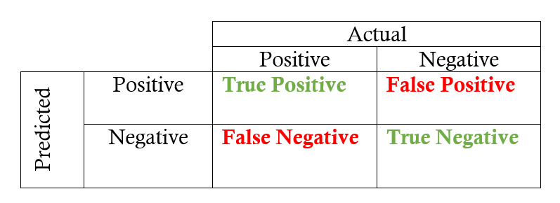
image from Towards Data Science
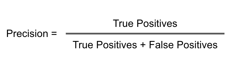
Precision
It is a classification metric use to evaluate the fraction of true positive predictions(TP) with respect to the total number of positive predictions(TP + FP) made by our model.
Recall
It evaluates the fraction of true positive predictions(TP) made by our model with respect to the actual number of positive examples(TP + FN) originally in our training dataset.
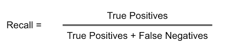
It is clear that, a dataset with far greater negative examples could result in a very low recall.
By changing the threshold value for the hypothesis function of a logistic classifier. i.e, hypothesis > threshold, we can obtain different values for precision and recall on the cross-validation set.
High precision and recall means learning algorithm performance is good
Which Classifier is Better?
To choose which classifier is best, based on precision and recall values, we often evaluate the average of precision and recall i.e (P + R) / 2. However, this is not a great way to decide which model is best as either a high precision and low recall or low precision and high recall of a particular model can lead to a high average value, whereas the model isn’t good.
F1-Score
To solve this drawback of the average evaluation, we use the F1-Score evaluation metric which is calculated as follows;
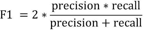
So if either precision or recall is very low, F1-score will be low. A high F1 score is only achieved by relatively high precision and recall. The best model has the highest F1 score.
DAY 6 DONE!!
** DAY 7 HIGHLIGHTS **
Support Vector Machines.
SVM is another interesting type of classifier similar to logistic regression with respect to its cost function. SVM’s don’t suffer from local minima problems as it’s cost function is purely convex.
SVM hypothesis and cost function are shown below:
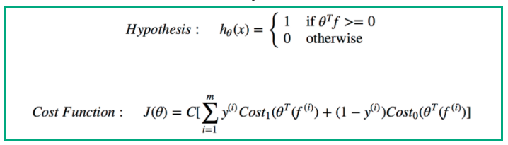
The objective of the SVM is to compute the best values of the model parameters(Thetas) that minimize the cost function — J(theta).
The hyperparameter, C in the cost function, which plays a role of C = 1 / lambda in the case of linear regression regularized cost function.
This means that, if C is large, lambda is very small and hence, model parameters are penalized less, leading to high-complexity and therefore overfitting. If C is small, lambda becomes large, resulting in high penalization of the model parameters which decreases model complexity leading to underfitting.
The hypothesis of SVM outputs a 1 for positive class and zero for the negative class directly. This is converse to Logistic regression which outputs a probability (0 to 1).
Developing Complex Non-Linear SVM Models
Similarity functions also known as Kernels can be used with SVMs to develop complex non-linear SVM models.
For example, the Gaussian kernel is a very common kernel that is based on selecting random points called landmarks on our training datasets and then, generating new features, k, based on the gaussian distribution equation.
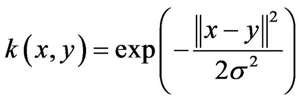
Gaussian kernel Function
y = vector of random landmarks and x = training example.
Based on the number of landmarks, for each training example, we evaluate k, then use that in our hypothesis to train and predict our model.
The idea of using kernels is just to create new features using our original training examples then train an SVM classifier using these new features instead of the original training dataset features.
Landmarks are usually selected at the same position as the training examples. Hence, if your training set has m examples, then you have m number of landmarks.
This results in a new feature vector k, of length m + 1, and consequently, your model will have model parameters (theta) of the same size as k, i.e m + 1. This includes the intercept term(theta-zero).
The new hypothesis then becomes:
predict, y = 1 , if (Theta * K > 0) and not the formal (Theta * X > 0)
Kernels can be used with linear regression but this is computationally expensive and should not be used unless absolutely needed.
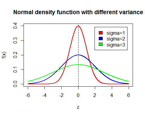
Image by VRC Academy
Another hyperparameter of SVMs is sigma in the gaussian kernel function. Large sigma results in a gentle sloping gaussian curve corresponding to low variance and high bias as the features k, vary smoothly. Small sigma, results in a steeper gaussian function, leading to high variance, and consequently, low bias as the features k, vary sharply.
Using SVMs with very large datasets is computationally expensive as the number of new features created using kernel equals the size of dataset examples.
For Multi-classification using SVM, we use the one-vs-all method to distinguish between the different classes. if we have K-classes, we simply train K SVM classifiers for each class by setting the corresponding class to y = 1, and all other classes to y = 0.
Prediction on an example is done by choosing SVM with the highest hypothesis value.
Key Note.
When to use SVM or Logistic Regression Classifier.
If the number of features, n is relatively larger than the number of training examples, m, for example, n = 10000, m = 10–1000, use logistic regression or SVM with no kernel.
If the number of features n is small, and m is intermediate e.g (n = 1–1000, m = 10–10000), use SVM with Gaussian kernels.
If n is small and m is very large e.g (n = 1 -1000, m = 50000+), it’s smart to use logistic regression or SVM with a linear kernel.
For all the above cases, neural networks tend to work well. Just a little bit slower.
If you want to get into greater detail, Savan wrote a great article on Support Vector Machines here.
DAY 7 DONE!!
** DAY 8 Highlights **
Unsupervised Learning.
In unsupervised machine learning, the model is fed with unlabeled data. It is up to the algorithm to find hidden structures, patterns, or relationships in the data.
Clustering algorithms are commonly used for unsupervised machine learning tasks.
K-means clustering algorithm is the most used clustering algorithm. It is used to get an intuition about the structure of the data.
The algorithm is iterative and is based on 2 main steps.
- Cluster Assignment step which assigns training examples to each cluster based on proximity of training example to cluster centroid.
2. Move cluster centroid step which relocates each centroid to the average or mean of its cluster subset.
Steps of K-Means Algorithms
The way the K-means algorithm works is as follows:
1. Specify the number of clusters K.
2. Initialize centroids by first shuffling the dataset and then randomly selecting K data points for the centroids without replacement.
3. Keep iterating until there is no change to the centroids. i.e assignment of data points to clusters isn’t changing.
4. Compute the sum of the squared distance between data points and all centroids.
5. Assign each data point to the closest cluster (centroid).
6. Compute the centroids for the clusters by taking the average of all data points that belong to each cluster.
The initialization of cluster centroids is done by assigning k-cluster centroids to randomly chosen k-training examples.
Dimensionality Reduction
It is another type of unsupervised learning algorithm. The most common dimensionality reduction algorithm is Principal Component Analysis(PCA)
PCA aims at finding a lower k-dimensional feature hyperplane (surface) on which to project the training examples of higher-dimension in such a way as to minimize the squared projection error(distance from each training example to the projection surface)
In choosing the number of principal components k for PCA, it is good practice to choose the smallest value of k for which 99% of the variance is retained.
We also apply PCA in supervised learning problems that have a very large number of features. This is applied only to the input training set of your dataset and not on the cross-validation or test set of the dataset.
PCA finds a mapping from training example x(i) to z(i), where z(i) is the new feature vector obtained after running PCA. So PCA can be considered a preprocessing step for supervised learning algorithms.
Main Applications of PCA
1. Compression: To reduce the memory/disk space used to store data and speed up learning algorithms.
2. Visualization applications where the number of principal components k can be either 1, 2, or 3 for easy visualization.
For more in-depth information on Dimensionality reduction here is a great resource on GeekforGeeks
DAY 8 DONE!!
** DAY 9 HIGHLIGHTS **
image from Coursera
Building an Anomaly Detection System
Anomaly Detection in machine learning is used to predict rare occurrences in our dataset which differs significantly from the majority of the data.
Its main application is in Fraud detection where we use our unlabeled dataset to build a probabilistic model. Then use that to detect any abnormal or fraudulent activities.
Manufacturing also uses Anomaly detection to determine if their products are faulty or not. Monitoring computers or servers in a data center is also another area where we see the use of anomaly detection applied.
Gaussian distribution is used for anomaly detection where we estimate
the mean and variance of the distribution using the training set data.
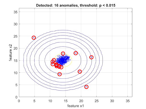
Image by SpLabs
Generally in an anomaly detection algorithm, we estimate the average(mean) and variance of individual features in our training dataset which becomes the model parameters.
Given a new example,x, we simply compute the probability, p(x) using the estimated mean and variance of the Gaussian distribution parameters obtained during training.
If p(x) < epsilon, then the example, x, is anomalous, otherwise, it is a normal condition.
The probability, p(x) is calculated based on the assumption of the independence of features. i.e p(x) is the product of the probability of each feature in the feature vector.
P(x) = P(x1)P(x2)P(x3)……..P(xn)
In building Anomaly detection systems, the dataset is often skewed as we usually have far more negative examples than positive. So, we recline from using classification accuracy as a performance metric which can be very high and misleading. It’s preferable to use the F1-score metric.
When to use Anomaly Detection Technique.
We use Anomaly detection instead of supervised learning algorithms when we have very very few positive examples (anomalous) and lots of negative examples(normal). This is because supervised learning will make it more challenging for the learning algorithm to learn from such a small subset of examples.
When interested in capturing some correlation between features we
can use a multivariate Gaussian model to estimate the parameters(mean vector and covariance matrix).
Recommender Systems
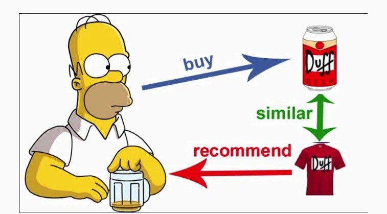
image from towards data science
The purpose of a recommender system is to suggest relevant items to users.
There exist two main categories of recommender systems: Content-based and collaborative filtering recommender systems.
Content-Based Recommender System
Let’s say for example we have collected information on the ratings given by users after watching certain movies on our website. The recommender system takes this information and tries to predict the possible rating value a user could have given to a movie he hasn’t watch yet.
Based on the estimated rating value, the system decides to suggest propose this movie to you. So in content-based recommender systems, we use additional information about our users and/or items.
Collaborative Filtering Recommender systems
This method is used to automatically learn relevant features for a recommender system.
The collaborative filtering algorithm’s objective is to use the ratings for every customer(user) and learn a set of features X, which it then uses to learn the model parameters for each user. With these parameters. Based on these learned features X, and parameters, thetas, the recommender can predict the ratings for products e.g movies without any ratings.
Also, the learned parameters can be used to compare features of the different movies and based on difference and then recommend new movies to its users.
Here is an article for more information regarding the collaborative Filtering algorithm.
Key Note
In a recommender system, each user has its own unique set of model parameters (thetas). So the number of users equals the number of linear regression models that have to be trained.
Mean Normalization is sometimes used to enhance the performance of the model especially when there exist users without no ratings for products.
For more information, here is an article by Baptiste Rocca on Recommender systems
DAY 9 DONE!!
** DAY 10 HIGHLIGHTS **
Large Scale Machine learning
As the size of the training dataset increases to millions of examples, gradient descent i.e batch gradient descent algorithm for finding the best model parameters becomes very inefficient due to the high computational time involved.
Stochastic Gradient Descent(SGD) algorithm is preferred in such cases as it is much faster. In the SGD algorithm, we first of all shuffle training data, then for each training example, we update the model parameters.
This is contrary to batch gradient descent where a single update of model parameters involves using all training examples.
Mini-batch gradient descent uses a mini-batch of our training dataset in each iteration to update model parameters. Contrary to SGD that uses a single example in each update iteration.
Map Reduce — Data parallelism Approach
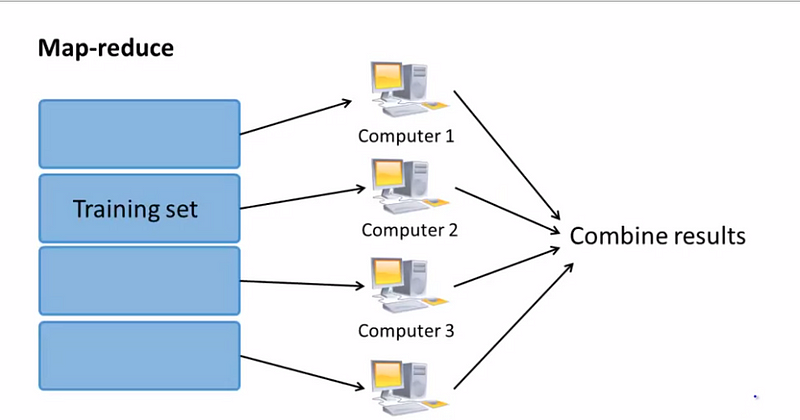
In the map-reduce approach, a very large training dataset in the ranges of hundreds of millions of examples is split into equal size subsets which can then be fed to different machines.
This allows for simultaneous computation of the partial sum over a subset. A centralized machine then combines the results from these multiple computers and then performs model parameter updates.
This reduces the time taken for learning model parameters. Map-reduce is also possible for multicore machines, where data parallelism is done across the different cores.
For more information on MapReduce check this out
DAY 10 DONE!!
** DAY 11 HIGHLIGHTS **
Machine Learning Pipeline
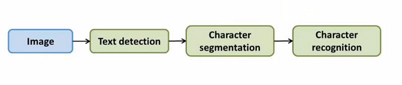
Typical machine learning pipeline
Application of machine learning problems generally follows a pipeline such as the example of a photo OCR(optical character recognition) shown above. The output from each block becomes the input into the next block.
Getting lots of data by artificial synthetic methods is a technique thatcan help improve the performance of your model only when the model has low bias. Low bias can be seen via plotting learning curves.
Key Note
For machine learning problems it is important to first check using Learning
curves if your model is suffering from low bias. Then second, ask the question, what will it take to get 10-times more data than what you currently have? And then you can engage in generating new datasets.
Ceiling analysis
It is the process of manually overriding each component in your system to provide 100% accurate predictions with that component. Thereafter, you can observe the overall improvement of your machine learning system component by component. This helps to determine which component of the pipeline you need to spend time improving.
More information on ceiling analysis can be found here
FINALLY DAY 11 DONE!!
Conclusion
In this article, I have presented in a structural and chronological manner the main ideas, concepts, and best practices of machine learning.
It highlighted the most important concepts of every day for all eleven(11) days while minimizing the technicalities of linear and multivariate calculus involved in machine learning.
I know this article is not exhaustive and could not cover in-depth most of these concepts, so I have provided links within the article for those interested in further reading.
If you are interested in learning more about machine learning, I encourage you to do so by registering for Andrew’s machine learning course. It will be worth your time and effort. Here is a link to the course on Coursera. The course helped me to structure this post.
Thanks for Reading!
If you found this article helpful feel and will love to show your support, then
- You can follow me on Medium here.
- Follow me on LinkedIn here.
- Visit my website; beltus.github.io for more interesting posts.
- Follow me onTwitter


Leave a comment